Lane Detection

In a nutshell, I’ve taken the following steps to accomplish this:

• Correct for Camera Distortion
• Filter Lane Pixels
• Get the“Sky View”
• Fit the “Best-Fit” Curve
• Project the Lane back to the “Vehicle-View” Image

1. CAMERA CALIBRATION

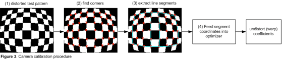
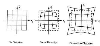
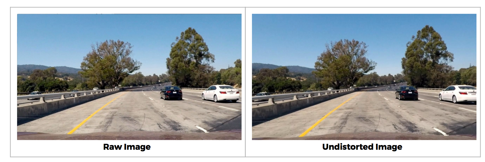
Because of the physical properties of a camera lens, the captured two-dimensional image isn’t perfect. There are image distortions that change the apparent size and shape of an object. More importantly it makes some objects appear closer or farther away than they actually are. Fortunately, we can measure this distortions and correct them. We can extract all the distortion information we need by having pictures of objects which we know where the certain points should be theoretically. Commonly used are chessboards on a flat surface because chessboards have regular high contrast patterns. It’s easy to imagine what an undistorted chessboard looks like.

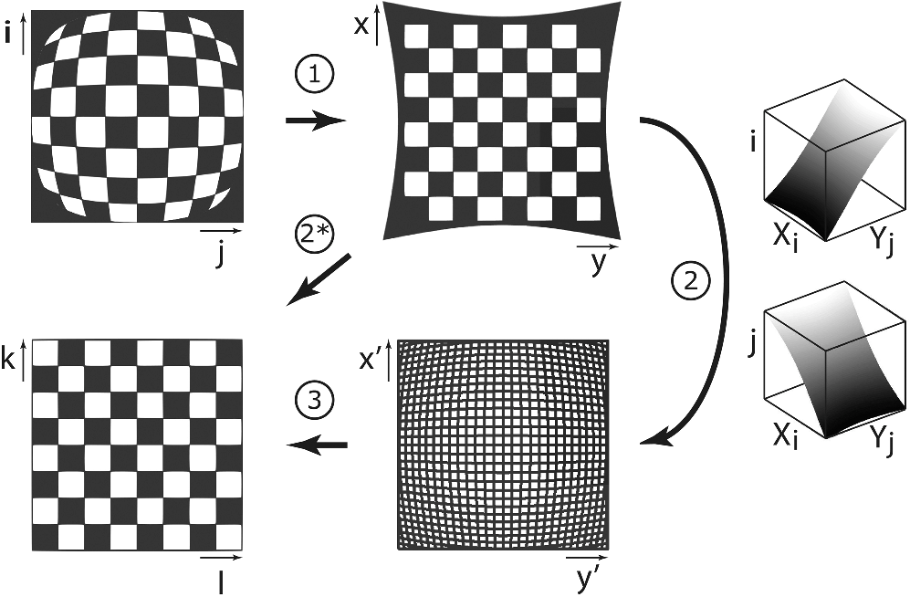
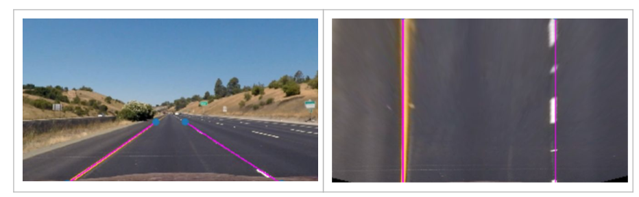
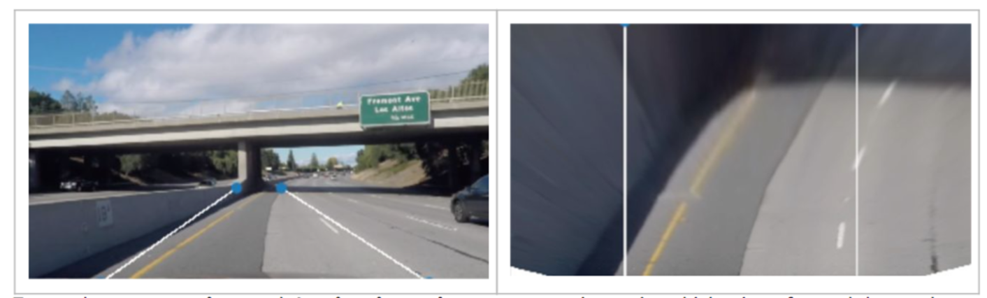
2. PERSPECTIVE TRANSFORMATION

After having the image corrected, we’d have an undistorted image of a road from the perspective of a vehicle. We can transform this image to an image of the road from the perspective of a bird in the sky. To extract all the information we need to warp this image from a vehicle view to sky view, we just need location coordinates. Specifically, all we need is one image which we have some locations from the input perspective (vehicle view) and the respective locations of the desired perspective (sky view). I call these location coordinates the source points and destination points. An easy image that we can “eye-ball” the correctness are straight parallel lines. What’s also great about this is we also have the information we need to warp from sky-view to vehicle-view as well.

3. GRADIENT AND COLOR THRESHOLDING

To estimate the curvature of a road, we don’t need all the information from all the pixels of a road image. The road lane lines from the video stream are yellow and white so we can mask everything out except the yellows and whites of the image. As an added precaution, because we might see some yellow and while lines that are not lanes, or there might be lanes which are not that distinctly yellow and white, we use what is called a Sobel operator. A Sobel operator essentially measures the rate of change in value (and its direction) between two locations of the image. This is also technically called as the derivative or gradient. More on this later.

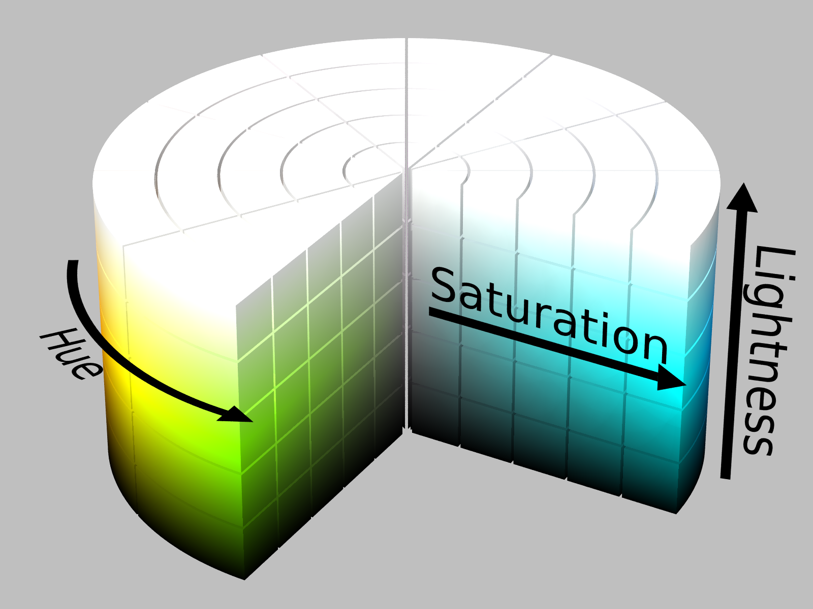
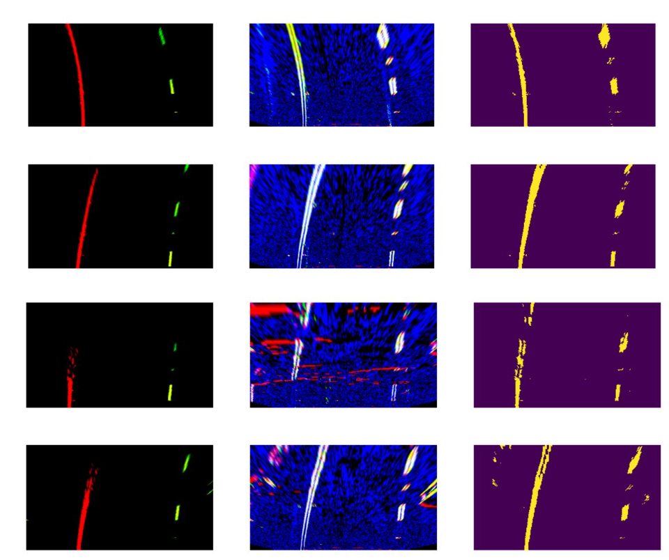
I represented the colors in HSL format. The Hue value is its perceived color number representation based on combinations of red, green and blue. The Saturation value is the measure of how colorful or or how dull it is. Lightness is how closer to white the color is. The yellow lanes are nicely singled out by a combination of lightness and saturation above a certain value. The white lanes are singled out by having a really high lightness value regardless of the saturation and hue.

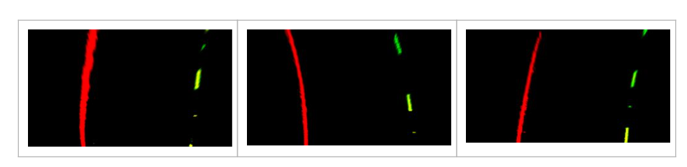
I applied the Sobel operator to the lightness value of the image. We used a combination of thresholding the gradient of the horizontal component, the magnitude of the gradient, and the direction of the gradient. I want to weed out locations of gradient that don’t have a large enough change in lightness. Thresholding the magnitude of the gradient as well as the x component of the gradient does a good job with that. I also only consider gradients of a particular orientation. A little above 0 degrees (or about 0.7 in radians), and below 90 degrees (or about 1.4 in radians). Zero implies horizontal lines and ninety implies vertical lines, and our lanes (in vehicle view) are in between them.

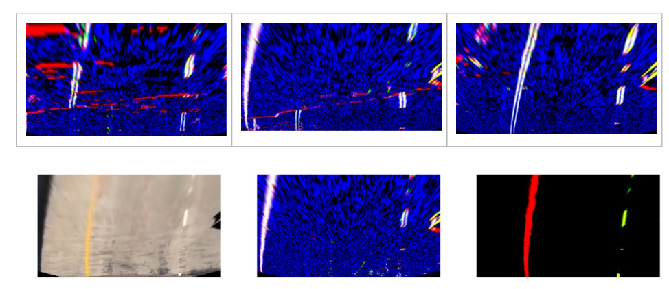
Adding both results of color and gradient thresholding filters out the lane lines quite nicely. We get some extraneous values from the edges of the image due to shadows, so mask them out afterwards.

4. CURVE FITTING

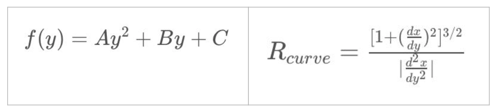
We can fit a curve for each lane line with a second degree polynomial function x = y² + By + C . We have to find the coefficients for each lane [A, B, C]. We can use the builtin function polyfit() All we have to do is feed it points and it outputs the coefficients of a polynomial of a specified degree of the curve that best fits the points fed.

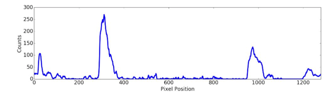
To decide which pixels are part of a lane, let’s implement this basic algorithm. I can take the histogram of all the columns of the lower half image and I will get graph with two peaks similar to the graph above. The prominent peaks of the histogram are good indicators of the x position of the base of the lane. So I use them as a starting point.

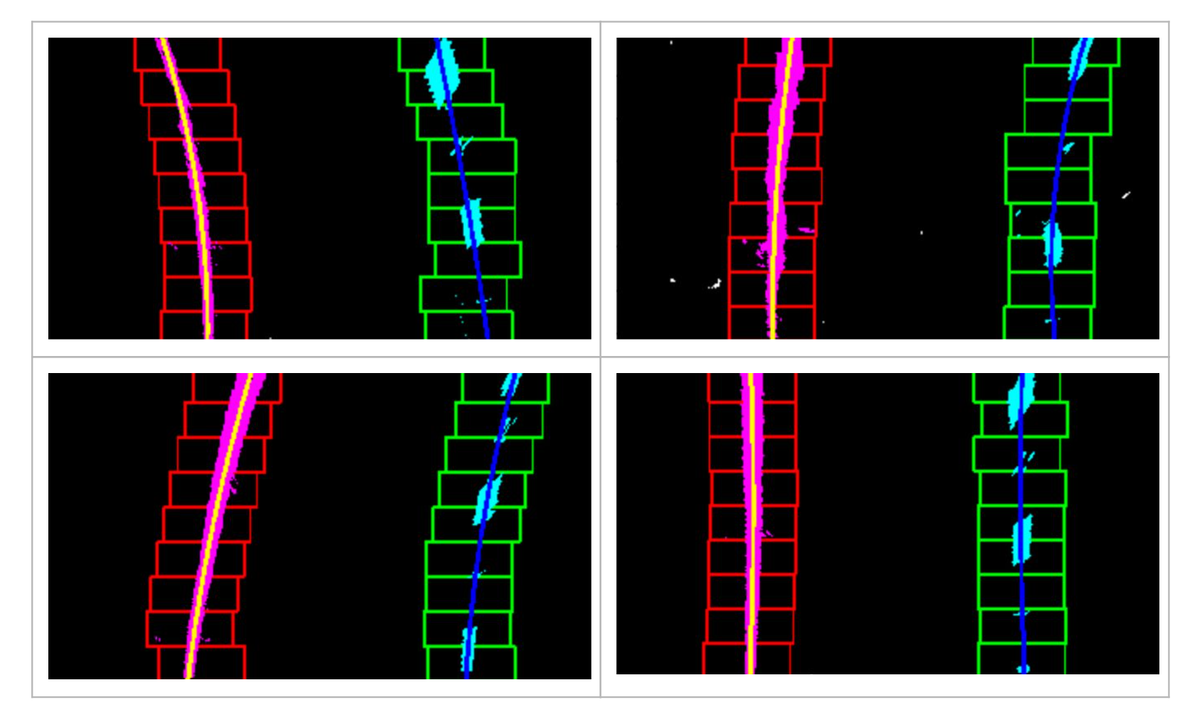
I can do a “sliding window technique” — one window on top of the other that follows the lanes up the frame. The pixels inside a “window” are marked as “pixels of interest” and added to the list of points in the lane. We average the x values of these pixels to give a good indication of the base point of the next window above. We can repeat this over and over until we get on top the lane. This way we have accumulated all the pixels that we are interested in that we will feed to our polyfit() function which spits out the coefficients of the 2nd degree polynomial. We can get compute the radius of curvature of each lane lines when we know the equations of the curve.

To estimate the vehicle position, I can calculate the lane width in pixels at the bottom of the image (closest to the camera). Say this was 1000 pixels wide. That implies that each pixel corresponds to 3.7 meters in real scale. Then I could compute the number of pixels the image center is offset from the lane center and interpolate the offset in meters.

5. LANE PROJECTION TO VEHICLE’S VIEW

Nice! We’ve actually gathered a lot of information about the road given a single image of the road. As I’ve said earlier in the Perspective Transformation section, we can use the same information to warp an image from sky-view to vehicle-view.

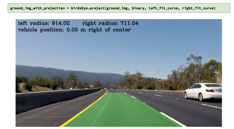
Because we now have the lane line curves parameters we get the points of the curves and the fillPoly() function to draw the lane region onto an image. We can now project our measurement down the road of the image. We wrap this up nicely in a neat little function calledbirdsEye.project()